Derivation of the Back Propagation Update Rule
A multilayer perceptron is a simple, artificial neural network. It bears little resemblance to biological neuronal networks, but has a surprising computational capacity. The multilayer perceptron is differentiated from the original perceptron in that it includes one or more “hidden” layers of neurons. A simple example looks like this:
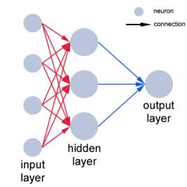
When the current state of the inputs is sent to the hidden layer, each hidden neuron computes a weighted sum of the entire input set. Then, based on a function of this weighted sum, the hidden neurons determine their current state. Then the output neuron computes a weighted sum of the states of the hidden neurons and determines the net output of the network by a function of the weighted sum.
When the network learns with a supervised learning algorithm like backpropagation, this output is then compared to the desired output (provided by the supervision, which gives a desired output for a given input). The difference between the two is calculated, and then this error is used to change the weights in the network in a way such that the error is minimized.
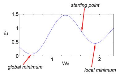
In practice, the square of the error is minimized. Additionally, the learning is throttled by a learning rate. This is for several reasons, but a key one is so that the network can be influenced by several different input patterns, not just the most recent one. If learning is not throttled, then the network loses the ability to minimize the error for many different input patterns and can only minimize the error on the most recently presented input pattern. Also note that this backpropagation algorithm only searches for a local minimum of E2, not a global minimum.
Terminology
network output = the state of the output neuron(s)
required output = the desired output state defined by the supervision, fixed for a given input pattern
input pattern = the state for the input neuron(s)
network output – required output = E = error
Abbreviations
E2 = squared error
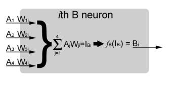
Ai = the state of the ith A neuron
WiB = the weight of the ith neuron to neuron B
IB = the weighted sum of all inputs to neuron B
Bi = the state of the ith B neuron
fB() = the activation function of neuron B, as a function of net input
η = the learning rate, it can range anywhere between 0 and 1, but is typically much less than 1
Loose analogies to biological neuronal networks
Calling the individual mathematical elements in the network “neurons” is convenient, though they share only a few abstract features with biological neurons. To press the analogy to its limit, here are some other loose analogies to biological neuronal networks.
Ai = voltage of the ith A neuron which is presynaptic to the B neurons
Bi = voltage of the ith B neuron which is postsynaptic to the A neurons
WiB = the strength of the synapse from the ith A neuron to the B neuron
IB = net synaptic current into a neuron B
fB() = the voltage response of the B neuron, as a function of net input current
Note:
Neuron A may be an input neuron or hidden layer neuron, but it is not the output neuron.
Neuron B may be an output neuron or a hidden layer neuron, but it is not the input neuron.
The state of each input neuron is determined by the input pattern. After the input layer, the state of each neuron in the network is determined as described above. Specifically, the state of neuron B is a function of the weighted sum of its inputs from the A layer.
Since,
 (1)
(1)
 (2)
(2)
The function fB can take many different forms. Some typical examples are:
Linear:
fB(x) = x
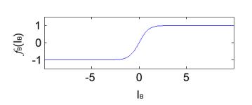
Hyperbolic
tangent: fB(x) = tanh(x)
Logisitic:
fB(x) = (1+e-x)-1
The hyperbolic tangent activation function looks like this:
After the output of the network (the state of the output neuron) is computed, is compared with the required output from the supervisor and the difference between the two values is squared to yield E2. In order to minimize this error, the weights in the network are each changed based on the partial derivative of the E2 with respect to the weight being changed.
 (3)
(3)
When the partial derivative term is negative, then the E2 function has a locally negative slope. In that case E2 is decreasing as WiB increases, so WiB grows to minimize E2. Similarly, when the partial derivative is positive, WiB decreases to minimize E2.
Now, to calculate that partial derivative for a particular WiB, call it WaB, where a=1, 2, or 3, the chain rule is used.
 (4)
(4)
and the last partial derivative in that equation can be simplified like this
 (5)
(5)
since only one term in IB is a function of WaB.
Substituting (4) and (5) into (3),
 (6)
(6)
This is the update rule. Most of the symbols on the right side are either picked a priori (η) or are kept track of automatically (WIB,old,Aa). However, the remaining partial derivative needs to be expressed in different terms. In order to do this, we will separately consider two possible cases:
1) Neuron B is in the output layer.
2) Neuron B is in the hidden layer.
In case 1, neuron B is an output neuron. Call its state B0. The network output in this network, which has a single output neuron, is defined as the state of that single output neuron. Therefore we can greatly simplify the update rule.
 (7)
(7)
Now the partial can be written as
 (8)
(8)
Since the required output has no dependency on IB. Notice that this last partial is simply the first derivative of the activation function of neuron B. Therefore,
 (9)
(9)
And the update rule becomes
 (10)
(10)
In case 2, neuron B is in the hidden layer. Then the partial derivative can be expanded in terms of IO, the weighted sum of inputs into the output neuron.
 (11)
(11)
But note,
 (12)
(12)
Additionally, when IO, the input into the output neuron, is expanded into the sum of inputs from the hidden layer, this relationship is obtained:
 (13)
(13)
where j counts all the neurons in the hidden layer, in this case layer B, and WjO is the weight between the jth hidden layer neuron and the output neuron. This can be further expanded and then simplified,
(14)
since most of the terms have no dependency on Bi. So then (11), using (12) and (14), can be rewritten:
 (15)
(15)
To summarize, for a neural network with one layer of hidden neurons between the input layer and the output layer, the weight update rule for a connection from neuron A to neuron B is:
 (16)
(16)
where
 if
neuron B is the output neuron
(17)
if
neuron B is the output neuron
(17)
 if neuron B
is a hidden neuron
(18)
if neuron B
is a hidden neuron
(18)
where fO and fh are the activation functions of the output layer and the hidden layer, respectively. Note that often the factor of 2 in (17) is absorbed into the learning rate, η.
Example with C++ source code
An example is shown at http://www.philbrierley.com/. The single example is shown in MATLAB, C, Fortran 90, PHP, and other flavors. Here I will walk through the example, this time for C++ in MFC using Visual Studio .NET.
Use the wizard to start a new MFC project. Make it a dialog application. Add a button to the dialog and then generate an event handler for when the button is pressed.
Assume a network as illustrated in figure 1, with three inputs, four hidden layer neurons, and one output. In this case, add these lines to the header file YourAppNameDlg.h, as public variables and functions:
CString str;
//// Data dependent settings
////
#define numInputs 3
#define numPatterns 4
#define numOutputs 1
//// User defineable
settings ////
#define numHidden 4
const int numEpochs;
const double LR_IH;
const double LR_HO;
//// functions ////
void initWeights();
void initData();
void calcNet();
void WeightChangesHO();
void WeightChangesIH();
void calcOverallError();
void displayResults();
double getRand();
//// variables ////
int patNum;
double
errThisPat[numOutputs];
double outPred[numOutputs];
double RMSerror[numOutputs];
// the outputs of the hidden
neurons
double hiddenVal[numHidden];
// the weights
double
weightsIH[numInputs][numHidden];
double
weightsHO[numHidden][numOutputs];
// the data
float
trainInputs[numPatterns][numInputs];
float trainOutput[numPatterns][numOutputs];
Now, in YourAppNameDlg.cpp, you need to alter the constructor so that a few variables are initialized.
Cnn2dualoutputDlg::Cnn2dualoutputDlg(CWnd*
pParent /*=NULL*/)
: CDialog(Cnn2dualoutputDlg::IDD, pParent),numEpochs(500),LR_IH(0.7),LR_HO(0.07)
And add these functions:
void
Cnn2dualoutputDlg::OnBnClickedButton1()
{
//// variables ////
patNum = 0;
for (int
m=0;m<numOutputs;m++) {
errThisPat[m]
= 0.0;
outPred[m]
= 0.0;
RMSerror[m]
= 0.0;
}
// seed random number
function
srand ( (unsigned
int)time(NULL) );
// initiate the weights
initWeights();
// load in the data
initData();
// train the network
for(int j = 0;j <=
numEpochs;j++) {
for(int
i = 0;i<numPatterns;i++) {
//select a pattern at random
patNum = rand()%numPatterns;
//calculate the current network
output
//and error for this pattern
calcNet();
//change network weights
WeightChangesHO();
WeightChangesIH();
}
//display
the overall network error
//after
each epoch
calcOverallError();
//printf("epoch
= %d RMS Error =
%f\n",j,RMSerror);
if
(j%100==0) {
str.Format("epoch = %d RMS
Error = %f,%f\n",j,RMSerror[0],RMSerror[1]);
AfxMessageBox(str);
}
}
//training has finished
//display the results
displayResults();
}
void
Cnn2dualoutputDlg::calcNet(void)
{
//calculate the outputs of
the hidden
neurons
//the hidden neurons are tanh
int i = 0;
for(i =
0;i<numHidden;i++) {
hiddenVal[i]
= 0.0;
for(int
j = 0;j<numInputs;j++) {
hiddenVal[i] = hiddenVal[i] +
(trainInputs[patNum][j] * weightsIH[j][i]);
}
hiddenVal[i]
= tanh(hiddenVal[i]); //
threshold is around 0
}
//calculate the output of
the network
//the output neurons are
linear
for (int
m=0;m<numOutputs;m++) {
outPred[m]
= 0.0;
for(i
= 0;i<numHidden;i++) {
outPred[m] = outPred[m] +
(hiddenVal[i] * weightsHO[i][m]);
}
//calculate
the error
errThisPat[m]
= outPred[m] -
trainOutput[patNum][m];
}
}
//************************************
//adjust
the weights
hidden-output
void
Cnn2dualoutputDlg::WeightChangesHO(void)
{
double weightChange;
for(int
m=0;m<numOutputs;m++) {
for(int
k=0;k<numHidden;k++)
{
weightChange = LR_HO *
errThisPat[m] * hiddenVal[k];
weightsHO[k][m] = weightsHO[k][m]
- weightChange;
//normalization on the output
weights
if (weightsHO[k][m] < -5)
weightsHO[k][m] = -5;
else if (weightsHO[k][m] > 5)
weightsHO[k][m] = 5;
}
}
}
//************************************
//
adjust the
weights input-hidden
void
Cnn2dualoutputDlg::WeightChangesIH(void)
{
for (int
m=0;m<numOutputs;m++) {
for(int
i = 0;i<numHidden;i++) {
for(int k = 0;k<numInputs;k++)
{
//double x = 1 -
abs(hiddenVal[i]);
//
works just as well
//double x = 1 -
(hiddenVal[i] * hiddenVal[i]); // original
double x = 1 - (hiddenVal[i]
* hiddenVal[i]);
//x = x * weightsHO[i] *
errThisPat * LR_IH;
x = x * weightsHO[i][m] *
errThisPat[m] * LR_IH;
x = x *
trainInputs[patNum][k];
double weightChange = x;
weightsIH[k][i] =
weightsIH[k][i] - weightChange;
}
}
}
}
double
Cnn2dualoutputDlg::getRand(void)
{
return
((double)rand())/(double)RAND_MAX;
}
void
Cnn2dualoutputDlg::initWeights(void)
{
for(int
j=0;j<numHidden;j++) {
for(int
i=0;i<numInputs;i++) weightsIH[i][j] =
(getRand() - 0.5)/5;
for(int
m=0;m<numOutputs;m++) weightsHO[j][m]
= (getRand() - 0.5)/4;//2;
}
}
void
Cnn2dualoutputDlg::initData(void)
{
AfxMessageBox("initializing
data");
// the data here is the XOR
data
// it has been rescaled to
the range
// [-1][1]
// an extra input valued 1
is also added
// to act as the bias
// the output must lie in
the range -1 to 1
trainInputs[0][0] = 1;
trainInputs[0][1] = -1;
trainInputs[0][2] = 1; //bias
trainOutput[0][0]=1;
trainOutput[0][1]=-0.5;
trainInputs[1][0] = -1;
trainInputs[1][1] = 1;
trainInputs[1][2] = 1;
//bias
trainOutput[1][0]=1;
trainOutput[1][1]=1;
trainInputs[2][0] = 1;
trainInputs[2][1] = 1;
trainInputs[2][2] = 1;
//bias
trainOutput[2][0]=-1;
trainOutput[2][1]=0.5;
trainInputs[3][0] = -1;
trainInputs[3][1] = -1;
trainInputs[3][2] = 1; //bias
trainOutput[3][0]=-1;
trainOutput[3][1]=0;
}
void
Cnn2dualoutputDlg::displayResults(void)
{
CString str2;
for(int i =
0;i<numPatterns;i++) {
patNum
= i;
calcNet();
str2.Format("pat
= %d actual =
%.1f,%.1f neural model =
%f,%f\n",patNum+1,trainOutput[patNum][0],trainOutput[patNum][1],outPred[0],outPred[1]);
AfxMessageBox(str2);
}
}
void
Cnn2dualoutputDlg::calcOverallError(void)
{
for (int
m=0;m<numOutputs;m++) {
RMSerror[m]
= 0.0;
for(int
i=0;i<numPatterns;i++) {
patNum = i;
calcNet();
RMSerror[m] = RMSerror[m] +
(errThisPat[m] * errThisPat[m]);
}
RMSerror[m]
= RMSerror[m]/numPatterns;
RMSerror[m]
= sqrt(RMSerror[m]);
}
}
A modification to include multiple outputs
CString str;
//// Data dependent settings
////
#define numInputs 3
#define numPatterns 4
#define numOutputs 2
//// User defineable
settings ////
#define numHidden 4
const int numEpochs;
const double LR_IH;
const double LR_HO;
//// functions ////
void initWeights();
void initData();
void calcNet();
void WeightChangesHO();
void WeightChangesIH();
void calcOverallError();
void displayResults();
double getRand();
//// variables ////
int patNum;
double
errThisPat[numOutputs];
double outPred[numOutputs];
double RMSerror[numOutputs];
// the outputs of the hidden
neurons
double hiddenVal[numHidden];
// the weights
double
weightsIH[numInputs][numHidden];
double
weightsHO[numHidden][numOutputs];
// the data
float
trainInputs[numPatterns][numInputs];
float trainOutput[numPatterns][numOutputs];
Now, in YourAppNameDlg.cpp, you need to alter the constructor so that a few variables are initialized.
Cnn2dualoutputDlg::Cnn2dualoutputDlg(CWnd*
pParent /*=NULL*/)
: CDialog(Cnn2dualoutputDlg::IDD, pParent),numEpochs(500),LR_IH(0.7),LR_HO(0.07)
And add these functions:
void
Cnn2dualoutputDlg::OnBnClickedButton1()
{
//// variables ////
patNum = 0;
for (int
m=0;m<numOutputs;m++) {
errThisPat[m]
= 0.0;
outPred[m]
= 0.0;
RMSerror[m]
= 0.0;
}
// seed random number
function
srand ( (unsigned
int)time(NULL) );
// initiate the weights
initWeights();
// load in the data
initData();
// train the network
for(int j = 0;j <=
numEpochs;j++) {
for(int
i = 0;i<numPatterns;i++) {
//select a pattern at random
patNum = rand()%numPatterns;
//calculate the current network
output
//and error for this pattern
calcNet();
//change network weights
WeightChangesHO();
WeightChangesIH();
}
//display
the overall network error
//after
each epoch
calcOverallError();
//printf("epoch
= %d RMS Error =
%f\n",j,RMSerror);
if
(j%100==0) {
str.Format("epoch = %d RMS
Error = %f,%f\n",j,RMSerror[0],RMSerror[1]);
AfxMessageBox(str);
}
}
//training has finished
//display the results
displayResults();
}
void
Cnn2dualoutputDlg::calcNet(void)
{
//calculate the outputs of
the hidden
neurons
//the hidden neurons are tanh
int i = 0;
for(i =
0;i<numHidden;i++) {
hiddenVal[i]
= 0.0;
for(int
j = 0;j<numInputs;j++) {
hiddenVal[i] = hiddenVal[i] +
(trainInputs[patNum][j] * weightsIH[j][i]);
}
hiddenVal[i]
= tanh(hiddenVal[i]); //
threshold is around 0
}
//calculate the output of
the network
//the output neurons are
linear
for (int
m=0;m<numOutputs;m++) {
outPred[m]
= 0.0;
for(i
= 0;i<numHidden;i++) {
outPred[m] = outPred[m] +
(hiddenVal[i] * weightsHO[i][m]);
}
//calculate
the error
errThisPat[m]
= outPred[m] -
trainOutput[patNum][m];
}
}
//************************************
//adjust
the weights
hidden-output
void
Cnn2dualoutputDlg::WeightChangesHO(void)
{
double weightChange;
for(int
m=0;m<numOutputs;m++) {
for(int
k=0;k<numHidden;k++)
{
weightChange = LR_HO *
errThisPat[m] * hiddenVal[k];
weightsHO[k][m] = weightsHO[k][m]
- weightChange;
//normalization on the output
weights
if (weightsHO[k][m] < -5)
weightsHO[k][m] = -5;
else if (weightsHO[k][m] > 5)
weightsHO[k][m] = 5;
}
}
}
//************************************
//
adjust the
weights input-hidden
void
Cnn2dualoutputDlg::WeightChangesIH(void)
{
for (int
m=0;m<numOutputs;m++) {
for(int
i = 0;i<numHidden;i++) {
for(int k = 0;k<numInputs;k++)
{
//double x = 1 -
abs(hiddenVal[i]);
//
works just as well
//double x = 1 -
(hiddenVal[i] * hiddenVal[i]); // original
double x = 1 - (hiddenVal[i]
* hiddenVal[i]);
//x = x * weightsHO[i] *
errThisPat * LR_IH;
x = x * weightsHO[i][m] *
errThisPat[m] * LR_IH;
x = x *
trainInputs[patNum][k];
double weightChange = x;
weightsIH[k][i] = weightsIH[k][i]
- weightChange;
}
}
}
}
double
Cnn2dualoutputDlg::getRand(void)
{
return
((double)rand())/(double)RAND_MAX;
}
void
Cnn2dualoutputDlg::initWeights(void)
{
for(int
j=0;j<numHidden;j++) {
for(int
i=0;i<numInputs;i++) weightsIH[i][j] =
(getRand() - 0.5)/5;
for(int
m=0;m<numOutputs;m++) weightsHO[j][m]
= (getRand() - 0.5)/4;//2;
}
}
void
Cnn2dualoutputDlg::initData(void)
{
AfxMessageBox("initializing
data");
// the data here is the XOR
data
// it has been rescaled to
the range
// [-1][1]
// an extra input valued 1
is also added
// to act as the bias
// the output must lie in
the range -1 to 1
trainInputs[0][0] = 1;
trainInputs[0][1] = -1;
trainInputs[0][2] = 1; //bias
trainOutput[0][0]=1;
trainOutput[0][1]=-0.5;
trainInputs[1][0] = -1;
trainInputs[1][1] = 1;
trainInputs[1][2] = 1;
//bias
trainOutput[1][0]=1;
trainOutput[1][1]=1;
trainInputs[2][0] = 1;
trainInputs[2][1] = 1;
trainInputs[2][2] = 1;
//bias
trainOutput[2][0]=-1;
trainOutput[2][1]=0.5;
trainInputs[3][0] = -1;
trainInputs[3][1] = -1;
trainInputs[3][2] = 1; //bias
trainOutput[3][0]=-1;
trainOutput[3][1]=0;
}
void
Cnn2dualoutputDlg::displayResults(void)
{
CString str2;
for(int i =
0;i<numPatterns;i++) {
patNum
= i;
calcNet();
str2.Format("pat
= %d actual =
%.1f,%.1f neural model =
%f,%f\n",patNum+1,trainOutput[patNum][0],trainOutput[patNum][1],outPred[0],outPred[1]);
AfxMessageBox(str2);
}
}
void
Cnn2dualoutputDlg::calcOverallError(void)
{
for (int
m=0;m<numOutputs;m++) {
RMSerror[m]
= 0.0;
for(int
i=0;i<numPatterns;i++) {
patNum = i;
calcNet();
RMSerror[m] = RMSerror[m] +
(errThisPat[m] * errThisPat[m]);
}
RMSerror[m]
= RMSerror[m]/numPatterns;
RMSerror[m]
= sqrt(RMSerror[m]);
}
}
Acknowledgements and References
The derivation of the backpropagation update rule presented here closely follows that of Phil Brierley. Furthermore, the source code in the examples derives from the source code of Brierley and dspink.
http://www.philbrierley.com/
Brierley P, (1998) Appendix A in "Some Practical Applications of Neural Networks in the Electricity Industry" Eng.D. Thesis, Cranfield University, UK.
Brierley P, Batty B, (1999) "Data mining with neural networks - an applied example in understanding electricity consumption patterns" in "Knowledge Discovery and Data Mining" (ed Max Bramer), chapter 12, INSPEC/IEE, ISBN 0852967675.